
Chilat Doina
August 26, 2026
The most popular advice in demand forecasting ecommerce is to buy a smarter model. That advice starts in the wrong place. An advanced algorithm can't reconcile duplicate SKUs, distinguish stockouts from zero demand, or understand that a returned item may represent demand that wasn't profitable to keep.
The operational question isn't, “Which AI model should we use?” It's, “Can our data and replenishment process turn a forecast into a stable purchase decision?” Global B2C ecommerce revenue is projected to reach USD 5.5 trillion by 2027, at a 14.4% compound annual growth rate, so small errors can become material inventory, cash-flow, and service-level problems at scale. (Journal of International Economics and International Commerce)
Most forecast failures happen before a model sees its first training row. Amazon, Shopify, and wholesale systems often use different identifiers, timestamps, inventory definitions, and refresh schedules. If the same product appears under several IDs, the model may interpret one demand stream as several unrelated products, while planners see phantom inventory or duplicate replenishment requirements.
A clean model can't repair a broken product master. Before comparing ARIMA with LightGBM, teams need to reconcile product identity, channel attribution, order status, cancellations, stockouts, transfers, and in-transit inventory. A forecasting-ready data warehouse architecture should make those definitions explicit rather than leaving them inside spreadsheets and individual analysts' workarounds. The data warehouse architecture guide is useful context for designing that shared foundation.
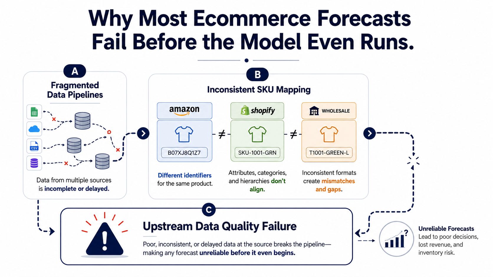
Fragmented feeds create silent gaps. Supplier lead times may arrive in a batch while marketplace orders update continuously. A stale feed can make available inventory look higher than it is, or make a demand drop look genuine when the channel stopped reporting.
Returns are often treated as an accounting adjustment instead of a demand signal. A high sales count may hide a recurring size, color, quality, or expectation mismatch. Forecasting gross sales without return propensity can cause a brand to buy more units of an item that produces weak net demand.
Replenishment instability appears when teams optimize a statistical score without testing order behavior. External variables can improve forecast accuracy while making purchase orders more volatile. In a study covering 4,523 products, external signals improved LightGBM accuracy by 15%, ESX by 6%, and Prophet by nearly 8%, while bullwhip increased by about 9% for LightGBM, nearly 9% for exponential smoothing, and over 31% for Prophet. (Digital Applied's ecommerce AI forecasting analysis)
Practical rule: A forecast is not production-ready until it has passed both an accuracy test and a replenishment-stability test.
A model can look highly accurate at the wrong horizon and still trigger a stockout before the next supplier delivery. Forecasting teams should align the horizon with the decision, then review outcomes with procurement, finance, merchandising, and fulfillment. The algorithm matters, but upstream definitions and operating agreement matter first.
Start with a canonical product record. Give every item one internal SKU, then map Amazon ASINs, Shopify product and variant IDs, wholesale UPCs, bundles, multipacks, and replacement items to that record. Preserve the channel identifiers for reporting, but never let a channel-specific ID become the product identity used by the forecasting layer.
Next, define the demand grain. Most replenishment decisions need demand by SKU, channel, location, and time period, with a clear distinction between ordered, shipped, cancelled, returned, and fulfilled units. Keep stockout periods visible. Zero sales while the product was unavailable isn't the same as zero customer interest.
The gross-demand layer records customer orders before returns. The returns layer captures returned units, reason codes, condition, refund status, and restockability. The net-demand layer then connects gross demand with returns, cancellations, and unusable inventory.
Promotional data belongs beside sales, not in a separate marketing report. Record campaign dates, channel, offer type, discount depth, audience, placement, and whether the promotion was planned or reactive. Shopify discount codes can obscure price response if the forecast sees only a sales spike and not the specific offer that caused it. Amazon promotions can also shift demand away from DTC, so the model needs channel context rather than treating each channel as independent.
Lead-time data deserves the same discipline. Store supplier, purchase order date, confirmation date, ship date, receipt date, promised lead time, actual lead time, and quantity received. Averages hide the risk that drives safety stock, especially when one supplier is consistently less reliable than another.
For teams building a broader analytics program, these real world retail big data examples show why the useful question is how operational signals connect, not how many dashboards a business has.
| Channel | Fragmentation Point | Impact on Forecast | Fix |
|---|---|---|---|
| Amazon | ASINs, FBA locations, marketplace promotions, and regional availability are separated | Regional demand can appear weaker or stronger than it really is | Map ASINs to canonical SKUs and retain location, promotion, and availability fields |
| Shopify | Product IDs, variants, discount codes, and returns may use different exports | Discounts can be mistaken for baseline demand, while returns distort net demand | Join orders, variants, promotions, and returns through a shared SKU key |
| Wholesale | UPCs, EDI batches, case packs, and delayed shipment confirmations use different timing | Demand may be recorded late or at the wrong unit of measure | Normalize units, preserve order dates, and separate requested from shipped quantities |
| Supplier data | Promised and actual lead times are often stored separately | Reorder points ignore delivery uncertainty | Store every purchase-order milestone and calculate lead-time variation by supplier and SKU |
The finished schema should make gross demand, returns, net demand, inventory position, stockouts, promotions, lead times, and channel attributes available in one time-series table. That structure supports statistical models, causal analysis, and machine learning without rebuilding the data every time the team changes methods. It also supports omnichannel inventory management, where the forecast must reflect one inventory position across several selling environments.
Model selection should follow the SKU's demand pattern and the decision horizon. A stable, high-volume replenishment item often benefits from exponential smoothing because recent demand carries useful information and the series contains enough observations to estimate a clean baseline. Complexity adds little if promotions, stockouts, and product identity are already handled well.
A promotional consumer-electronics SKU needs a different approach. If the item runs frequent weekly offers, a causal model can separate baseline demand from price and promotional effects. Regression is easier to explain to a buyer because the team can inspect how price, campaign timing, and lagged effects influence the result. Machine learning becomes more useful when those relationships are nonlinear or interact with channel, season, and inventory availability.
A seasonal apparel item with a recurring annual cycle needs explicit seasonal structure. Exponential smoothing with a seasonal component can be a strong starting point, while Prophet or another time-series model may help when holidays and trend changes are represented consistently. The model should operate at the SKU-channel level because one color or channel can peak differently from another.
A long-tail accessory with many zero-demand periods creates a sparse-demand problem. Standard percentage-error metrics and ordinary moving averages can behave badly when actual demand is zero or intermittent. Croston-style methods, intermittent-demand models, or a carefully designed pooled model can better separate demand occurrence from demand size.
A new product has no history to extrapolate. Use analogous SKUs, product attributes, price bands, category, channel, and launch context to establish an initial prior. Human review still matters, but the override should be documented as an assumption that can be measured after launch.
| SKU Type | Volume | Volatility | Best Model | Why |
|---|---|---|---|---|
| Core replenishment item | High and steady | Low | Exponential smoothing or a simple baseline | Recent demand usually provides a dependable signal |
| Promotional electronics | High | Medium to high | Causal regression or hybrid ML | Price, promotion, and lag effects need separate treatment |
| Seasonal apparel | Medium | Seasonal | Seasonal time-series or hybrid model | The model must preserve recurring cycles without baking promotions into baseline |
| Long-tail accessory | Low or intermittent | High relative to volume | Intermittent-demand method or pooled ML | Zero periods need different treatment from stable demand |
| New launch | Unknown | Unknown | Analogous or attribute-based model | Similar products provide a defensible starting point |
A useful benchmark is the SSA-BPNN neural-network model described in a cross-border ecommerce inventory study. It achieved 1.89% MAPE, 2.56% mean absolute error, 3.21 root mean square error, and an R2 value of 0.97 in that study, demonstrating what advanced modeling can achieve under a defined dataset and evaluation setup. (IJNRD inventory forecasting study) Those figures aren't a universal target for every catalog. They're evidence that model gains can matter when the data, SKU scope, and test design are appropriate.
For a broader overview of the trade-offs between baseline, time-series, causal, and machine-learning approaches, the sales forecasting methods guide provides a useful companion reference. Tune seasonality windows to the actual buying cycle, test promotion lags, and avoid fitting a short product lifecycle so tightly that the model memorizes launch noise.
Seasonality changes the baseline. Promotions create artificial spikes. New products remove the historical baseline altogether. Treating all three as ordinary variation causes the replenishment system to react late, order too much, or miss the first meaningful signal.
For seasonality, decompose demand at the SKU-channel level. A brand selling apparel through DTC, Amazon, and wholesale shouldn't use one blended seasonal index if each channel has different timing, assortment, and customer behavior. Separate trend, recurring seasonality, event effects, and availability constraints, then review whether the seasonal pattern remains stable after removing promotions.
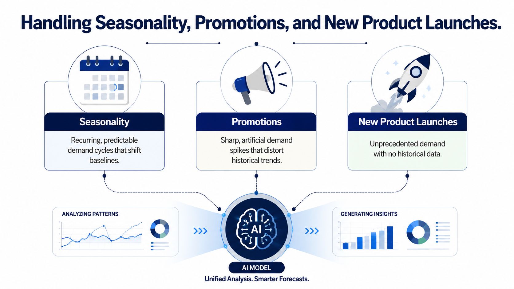
Black Friday illustrates the problem clearly. A DTC apparel brand may see customers pull purchases forward during the event, while related products are cannibalized and demand dips afterward. If the model carries the full spike into the following periods, the buyer replenishes against demand that already happened.
Record the promotion as an event with a start, end, offer, channel, and expected post-event behavior. Forecast baseline demand separately from incremental uplift, then test the recovery period. For Amazon, Prime Day can create a halo across parent-child ASINs, but the effect isn't necessarily equal across sizes, colors, or bundles. Parent-level reporting can hide the child SKU that needs replenishment.
Launches require priors rather than false precision. For a wholesale line extension with no direct comparable, cluster products by category, price, pack configuration, channel, and customer use case. Use the closest analogues to set an initial range, then update quickly as sales, search behavior, traffic, and returns arrive.
Operational test: If a promotion changes the forecast but leaves the purchase order unchanged, the model may be informative without being useful.
The inventory optimization guidance from Arlo Inc. offers additional context on connecting forecasting with stockout prevention and replenishment execution. The important discipline is to separate structural demand from temporary events, then put guardrails around how quickly the order plan can change.
MAPE is familiar, but it can become a distraction. Percentage-error metrics behave poorly for intermittent demand, and an aggregate score can conceal a forecast that overstates slow items while understating the products that drive service risk.
Evaluate accuracy at the SKU level and at the exact replenishment horizon. A monthly forecast may look strong for finance while failing the weekly purchase-order decision. Segment targets by demand pattern rather than forcing stable, seasonal, and volatile products into one benchmark. Practical WAPE guidance places stable repeat-purchase items around 10% to 20%, seasonal items around 20% to 35%, and volatile or trend-driven items above 35% even with strong models. (Ecommerce demand forecasting metrics guidance)
Track WAPE, bias, and forecast value added against a naive baseline. WAPE shows the size of the error across a portfolio, bias shows whether the team consistently over- or under-forecasts, and forecast value added shows whether a new model, planner override, or process step improves the result.
Then simulate the decision. Feed historical forecasts into the actual replenishment logic and calculate what would have happened to stockouts, excess inventory, inventory turns, working capital, and purchase-order volatility. A forecast that lowers error but causes buyers to swing orders sharply may increase the bullwhip effect and create more supply-chain cost.
| Metric Type | Statistical Metric | Operational Alternative | Why It Matters |
|---|---|---|---|
| Error size | WAPE or MAPE | Service-level impact by SKU class | Shows whether the forecast supports the products customers expect to find |
| Direction | Forecast bias | Excess and shortage exposure | Reveals systematic overbuying or underbuying |
| Large misses | RMSE | Expedite, markdown, or stockout consequences | Connects unusually bad errors with actual operating cost |
| Process contribution | Forecast value added | Override and workflow impact | Shows whether added human or model steps earn their complexity |
| Stability | Error volatility | Purchase-order volatility and lead-time sensitivity | Detects bullwhip risk that accuracy alone misses |
| Portfolio result | Aggregate score | Turns, working capital, and service outcomes | Prevents a good average from hiding SKU-level failures |
Backtesting should use rolling time splits, not random shuffling. Train on the past, forecast a future window that matches the replenishment horizon, advance the cutoff, and repeat. Keep promotions, stockouts, returns, and supplier delays in the historical simulation so the test reflects the conditions buyers face.
The best model isn't the one with the lowest error in isolation. It's the one that produces a better inventory decision without making the supply plan unstable.
Set thresholds by SKU velocity, margin, lead time, and channel importance. A hero item with long supplier lead time deserves tighter monitoring than a low-value accessory, even if the accessory has a worse percentage error. Review results weekly for fast-moving classes and monthly for slower groups, then investigate bias before adding model complexity.
A forecasting notebook proves that a method can run on prepared data. Production forecasting must survive delayed webhooks, marketplace API limits, wholesale batch files, inventory corrections, and manual overrides without losing traceability.
Use a layered serving design. Ingestion collects channel, order, inventory, return, promotion, and supplier data. Standardization validates identifiers and timestamps. Feature generation creates lagged demand, availability, promotional, and lead-time variables. The model service then writes forecasts with a version, run time, horizon, and confidence information into the replenishment system.
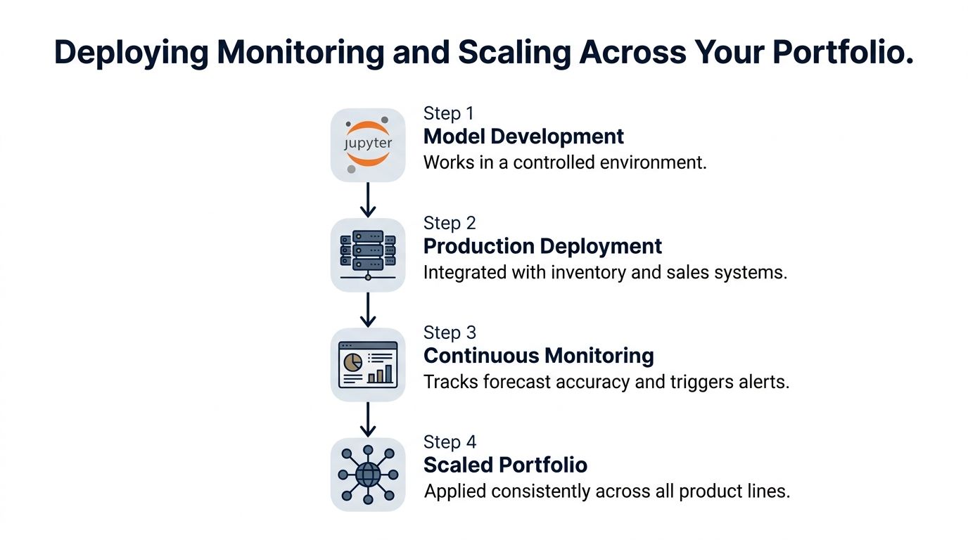
A sudden demand collapse may indicate a genuine market shift, but it may also mean that a Shopify webhook stopped arriving or an Amazon feed is stale. Monitor data freshness, row counts, missing SKU mappings, duplicate orders, inventory reconciliation, return-feed completeness, and supplier update timing alongside forecast error.
Alerts should reflect SKU criticality. A small deviation on a low-velocity accessory may need review during the next planning cycle. The same deviation on a high-volume item with a long lead time may require immediate intervention. Don't let one portfolio-wide threshold create either alert fatigue or dangerous silence.
Model governance keeps the process explainable. Store model versions, training windows, feature definitions, overrides, approval owners, and the final forecast used to generate each purchase recommendation. Merchandising teams should be able to override a forecast for a documented reason, such as a confirmed assortment change or supply constraint, while the system records whether that override improved the outcome.
For implementation detail on deployment, reproducibility, monitoring, and lifecycle controls, this practical MLOps guide is a useful technical reference.
A brand expanding from DTC into Amazon and wholesale shouldn't build three unrelated forecasting systems. Extend one canonical product and demand layer, then add channel-specific features, calendars, service rules, and data adapters. That approach preserves shared learning while respecting different fulfillment promises and replenishment cycles.
Million Dollar Sellers offers an operator community where ecommerce founders exchange practical strategies, including inventory forecasting approaches across Amazon, DTC, and omnichannel businesses. Visit Million Dollar Sellers to connect with experienced sellers and pressure-test your forecasting and replenishment decisions against real operating experience.
Join the Ecom Entrepreneur Community for Vetted 7-9 Figure Ecommerce Founders
Learn MoreYou may also like:
Learn more about our special events!
Check Events